Mapping Report of gi|549058243|emb|JB409847.1|
Report created with Sequana (0.1.16) and reports (0.3.0).
Sequencing depth and genome coverage report
Chromosome: gi|549058243|emb|JB409847.1|
Coverage
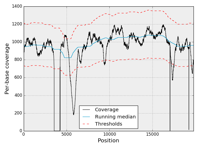
The following figure shows the per-base coverage along the reference genome
(black line). The blue line indicates the running median. From the normalised
coverage, we estimate z-scores on a per-base level. The red lines indicates the
z-scores at plus or minus N standard deviations, where N is chosen by the user
(default:4).
The image above is a static image. However, interactive plots are available from
the table here below. To allows interactions, we split the data into chunks of
500,000 bp length at max. The names contains the start and end positions.
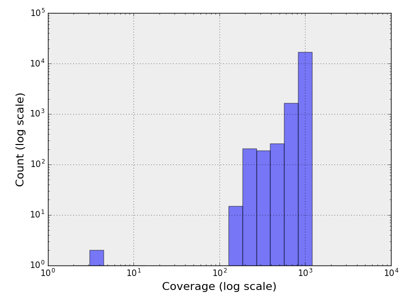
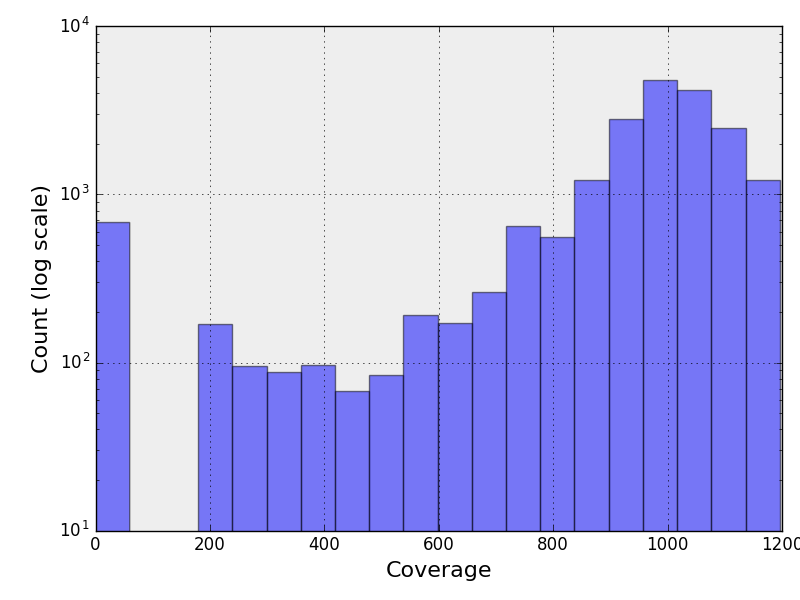
The following figure contains the histogram of the genome coverage. The X and Y
axis being in log scale.
Basic stats
The following table gives some basic statistics about the genome coverage.
| name | Value | Description |
|---|---|---|
| BOC | 96.60 | breadth of coverage: the proportion (in %s) of the genome covered by at least one read. |
| CV | 0.25 | the coefficient of variation |
| DOC | 931.31 | the sequencing depth (Depth of Coverage), that is the average ofthe genome coverage |
| MAD | 71.00 | median of the absolute median deviation median(|X-median(X)|) |
| Median | 988.00 | Median of the coverage |
| STD | 237.15 | standard deviation |
| GC | 48.42 | GC content in % |
Regions of Interest
Running median is the median computed along the genome using a sliding window. The following tables give regions of interest detected by sequana. Here is some captions:- mean_cov: the average of coverage
- mean_rm: the average of running median
- mean_zscore: the average of zscore
- max_zscore: the higher zscore contains in the region
Low coverage region
Regions with a z-score lower than -2.00 and at least one base with a z-score lower than -4.00 are detected as low coverage region. Thus, there are 8 low coverage regions| chr | start | end | size | mean_cov | mean_rm | mean_zscore | max_zscore |
|---|---|---|---|---|---|---|---|
| gi|549058243|emb|JB409847.1| | 3553 | 4252 | 699.0 |
24.59 | 917.63 | -15.77 | -16.20 |
| gi|549058243|emb|JB409847.1| | 5399 | 6212 | 813.0 |
401.34 | 877.59 | -8.84 | -12.93 |
| gi|549058243|emb|JB409847.1| | 9344 | 9561 | 217.0 |
766.71 | 1044.03 | -4.43 | -4.81 |
| gi|549058243|emb|JB409847.1| | 17045 | 17048 | 3.0 |
1.00 | 1007.00 | -16.18 | -16.20 |
| gi|549058243|emb|JB409847.1| | 17052 | 17053 | 1.0 |
4.00 | 1006.00 | -16.14 | -16.14 |
| gi|549058243|emb|JB409847.1| | 17186 | 17525 | 339.0 |
676.79 | 987.30 | -5.21 | -6.96 |
| gi|549058243|emb|JB409847.1| | 19257 | 19258 | 1.0 |
13.00 | 962.00 | -15.98 | -15.98 |
| gi|549058243|emb|JB409847.1| | 19554 | 19722 | 168.0 |
684.32 | 962.00 | -4.80 | -5.47 |
Download the CSV file
High coverage region
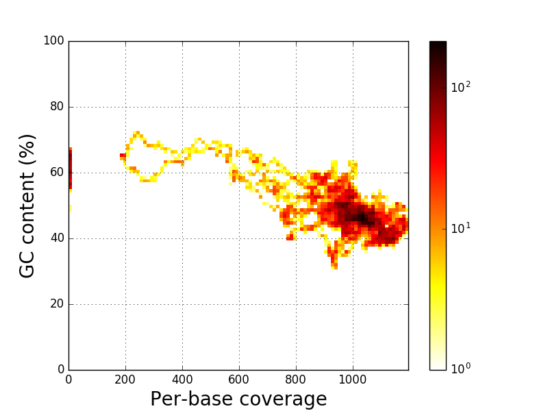
Regions with a z-score higher than 2.00 and at least one base with a z-score higher than 4.00 are detected as high coverage region. Thus, there are 1 high coverage regionsCoverage versus GC
Normalized coverage
Distribution of the normalized coverage with predicted Gaussian. The red line should be followed the trend of the barplot.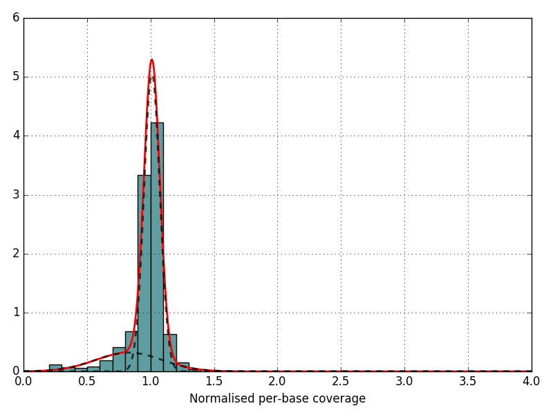
Z-Score distribution
Distribution of the z-score (normalised coverage); You should see a Gaussian distribution centered around 0. The estimated parameters are mu=1.01 and sigma=0.06.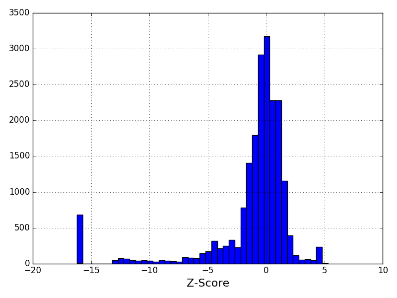
command used:
/home/cokelaer/anaconda2/envs/py35/bin/sequana_coverage --input JB409847.bed --reference JB409847.fa -o